Forecasting With Prophet

Not a cure-all for your all your forecasting ills

Not a cure-all for your all your forecasting ills
Author

Mike Aguilar

Published

April 6, 2026

I’ve spoken to several young researchers lately that are enamored with FB’s Prophet.

It’s a great model, but two things stand out to me:

  1. Philosophically, it’s more of a seasonal decomposition filter akin to ARIMA-SEAT-X13, than it is a forecasting model
  2. Despite it’s great power, it’s not a panacea.

Let’s play a little game by throwing Prophet at the task of forecasting daily stock returns. I’ll use the IVV. We can quibble about the sample period and ticker choice, etc… Acknowledged. But, for my young analysts, out there, take a look at what happens when you treat Prophet like a cure-all for all your forecasting ills.

Housekeeping

cat("\014")  # clear console
rm(list=ls())  # Clear the workspace
library(quantmod)
Loading required package: xts
Loading required package: zoo

Attaching package: 'zoo'
The following objects are masked from 'package:base':

    as.Date, as.Date.numeric
Loading required package: TTR
Registered S3 method overwritten by 'quantmod':
  method            from
  as.zoo.data.frame zoo 
library(prophet)
Warning: package 'prophet' was built under R version 4.5.3
Loading required package: Rcpp
Loading required package: rlang
library(dplyr)

######################### Warning from 'xts' package ##########################
#                                                                             #
# The dplyr lag() function breaks how base R's lag() function is supposed to  #
# work, which breaks lag(my_xts). Calls to lag(my_xts) that you type or       #
# source() into this session won't work correctly.                            #
#                                                                             #
# Use stats::lag() to make sure you're not using dplyr::lag(), or you can add #
# conflictRules('dplyr', exclude = 'lag') to your .Rprofile to stop           #
# dplyr from breaking base R's lag() function.                                #
#                                                                             #
# Code in packages is not affected. It's protected by R's namespace mechanism #
# Set `options(xts.warn_dplyr_breaks_lag = FALSE)` to suppress this warning.  #
#                                                                             #
###############################################################################

Attaching package: 'dplyr'
The following objects are masked from 'package:xts':

    first, last
The following objects are masked from 'package:stats':

    filter, lag
The following objects are masked from 'package:base':

    intersect, setdiff, setequal, union
library(ggplot2)
library(tidyr)
library(forecast)
library(zoo)

Data

Task: Gather the IVV’s adjusted closing from yahoo finance from 2010-01-01 through 2026-03-01. Construct log returns.

getSymbols("IVV", src="yahoo", from="2010-01-01", to="2026-03-01")
[1] "IVV"
prices <- Ad(IVV)
returns <- na.omit(diff(log(prices)))

Task: Create a simple dataframe of dates and returns.

df <- data.frame(
  ds = index(returns),
  y = as.numeric(returns)
)
n <- nrow(df)

Task: Create train, validation, and test periods, in that temporal order. Save the last 5 periods for testing, the 10 periods prior to the test period to be validation and the remaining to be training.

test_h <- 5
val_h <- 10

train <- df[1:(n - test_h - val_h),]
validation <- df[(n - test_h - val_h + 1):(n - test_h),]
test <- df[(n - test_h + 1):n,]

train_full <- rbind(train, validation)

Estimation

Full Seasonality Model

Task: Use “prophet” to estimate the Prophet model.

m_full <- prophet(
  train_full,
  growth = "linear",
  n.changepoints = 25,
  changepoint.range = 0.8,
  yearly.seasonality = FALSE,
  weekly.seasonality = TRUE,
  daily.seasonality = TRUE,
  seasonality.mode = "additive",
  seasonality.prior.scale = 10,
  changepoint.prior.scale = 0.05,
  interval.width = 0.80,
  uncertainty.samples = 0,
  algorithm = "Newton"
)

Task: use make_future_dataframe to create an object for predict test sample returns

future <- make_future_dataframe(m_full, periods = test_h)

Task: predict on the for the in sample and future dates

fc_full <- predict(m_full, future)

Task: Create a small object that captures the predictions only for the out of sample dates

pred_full <- tail(fc_full$yhat, test_h)

Forecast Evaluation

Task: Create an object callled pred_mean that is a simple mean prediction as a baseline.

mean_ret <- mean(train_full$y)
pred_mean <- rep(mean_ret, test_h)

RMSFE

Task: Construct the RMSFE for both models

rmsfe_full <- sqrt(mean((test$y - pred_full)^2))
rmsfe_mean <- sqrt(mean((test$y - pred_mean)^2))

data.frame(
  Model = c("Prophet Full", "Mean"),
  RMSFE = c(rmsfe_full, rmsfe_mean)
)
         Model       RMSFE
1 Prophet Full 0.007567685
2         Mean 0.007498113

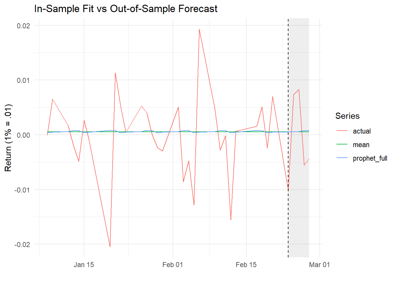
Task: Create a plot of the last 30 days of the full training period with the test period spliced onto that. Then create a plot of the actual data, prophet forecasts, and a simple full training period sample mean as a benchmark.

window_size <- 30

train_tail <- tail(train_full, window_size)
cutoff_date <- min(test$ds)

# ---- Extract fitted values (in-sample) ----
fit_full <- tail(fc_full$yhat[1:nrow(train_full)], window_size)

# ---- Mean (same in-sample and out-of-sample) ----
mean_line_train <- rep(mean_ret, window_size)
mean_line_test <- rep(mean_ret, test_h)

# ---- Combine data ----
plot_df <- data.frame(
  ds = c(train_tail$ds, test$ds),
  actual = c(train_tail$y, test$y),
  
  prophet_full = c(fit_full, pred_full),
  mean = c(mean_line_train, mean_line_test)
)

plot_long <- pivot_longer(plot_df, -ds)


ggplot(plot_long, aes(x = ds, y = value, color = name)) +
  
  # Shade test region
  annotate("rect",
           xmin = cutoff_date,
           xmax = max(plot_df$ds),
           ymin = -Inf,
           ymax = Inf,
           alpha = 0.1) +
  
  # Lines
  geom_line() +
  
  # 🔻 Train/Test split
  geom_vline(xintercept = cutoff_date, linetype = "dashed") +
  
  ggtitle("In-Sample Fit vs Out-of-Sample Forecast") +
  labs(
    color = "Series", 
    x = "", 
    y = "Return (1% = .01)"
  ) +
  theme_minimal()

EDA

Q: What did we do wrong? What should we always do first?

A: EDA. We SHOULD have done EDA first.

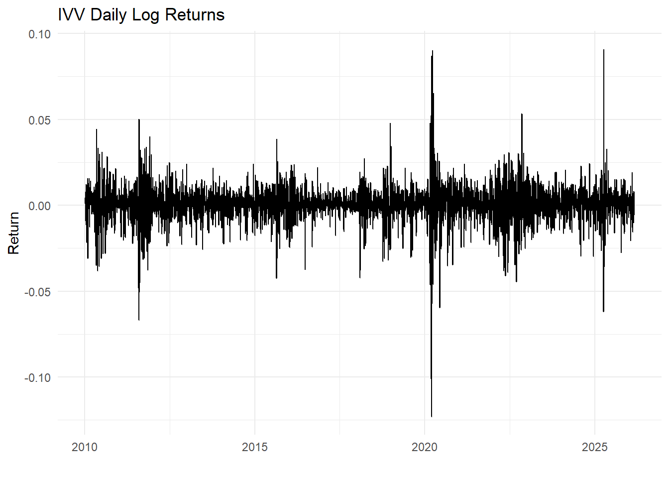
Task: plot the IVV over time

ggplot(df, aes(x = ds, y = y)) +
  geom_line() +
  ggtitle("IVV Daily Log Returns") +
  labs(x = "", y = "Return") +
  theme_minimal()

Q: Comment on the behavior as it relates to our modeling efforts.

A:

  • Mean 0
  • No trend
  • Little persistence

ACF

Task: Test for independence of the returns

Box.test(train_full$y, lag = 10, type = "Ljung-Box")

    Box-Ljung test

data:  train_full$y
X-squared = 200.48, df = 10, p-value < 2.2e-16

Q: Interpretation?

A:

  • H0: Independence of the returns over time
  • Small p value implies we reject
  • i.e. there is evidence of some temporal dependence

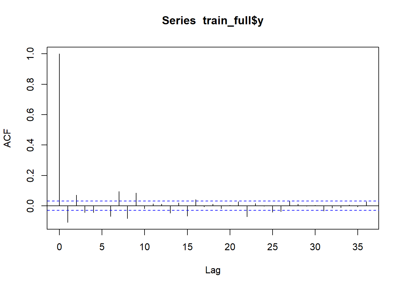
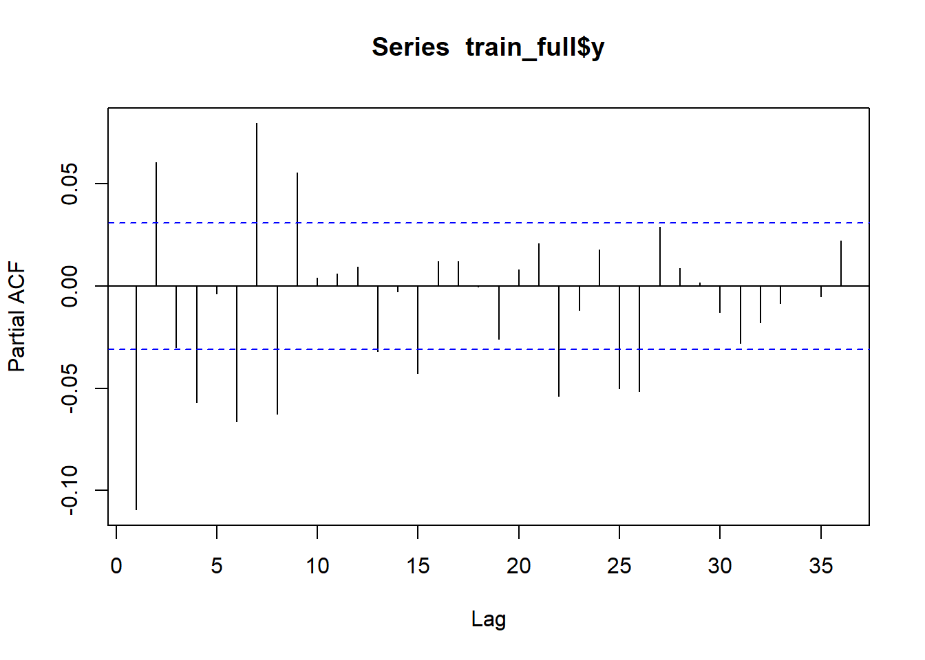
Task: Create the ACF and PACF

acf(train_full$y)

pacf(train_full$y)

Q: Interpret the plots.

A:

  • There are a few significant spikes, which is consistent with the Box test, but…
  • …the spikes are small in magnitude, and ….
  • …the spikes oscillate from positive and negative
  • These are usually signs of a lack of structural pattern

Seasonal Decomposition

Task: Convert train_full for a ts object

ret_ts <- ts(train_full$y, frequency = 252)

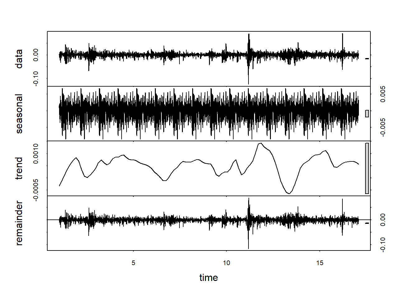
Task: Estimate STL and plot

stl_fit <- stl(ret_ts, s.window = "periodic")
plot(stl_fit)

Q: What does the plot suggest?

A:

  • There is little visible seasonality and not a strong linear time trend
  • Prophet relies on trend and seasonality. Since both are weak in returns, the model effectively collapses toward predicting the mean.
  • Minor note: The gray bars indicate the scale (amplitude) of each component within its own panel. They are not directly comparable to the original data scale and do not measure importance.

Task: Compute strength of trend and strength of seasonal

Strength of Trend = max(0,1-variance(noise)/var(Trend + noise))

Strength of Seasonal = max(0,1-variance(noise)/var(Seasonal + noise))

Tt <- stl_fit$time.series[, "trend"]
St <- stl_fit$time.series[, "seasonal"]
Rt <- stl_fit$time.series[, "remainder"]

F_trend <- max(0, 1 - var(Rt, na.rm=TRUE) / var(Tt + Rt, na.rm=TRUE))
F_season <- max(0, 1 - var(Rt, na.rm=TRUE) / var(St + Rt, na.rm=TRUE))

data.frame(
  Trend_Strength = F_trend,
  Seasonal_Strength = F_season
)
  Trend_Strength Seasonal_Strength
1    0.001917903        0.05801254

Q: Interpretation regarding seasonality and trend?

A:

  • Seasonal is stronger than trend
  • But these measures span from 0 to 1
  • The magnitude of the observed values support barely anything for Prophet to use to build a reasonable forecast.

Model Validation

Perhaps we’re being unfair to Prophet. Maybe we need to tune the model.

Task: Create a grid of hyperparameters for daily, weekly, and seasonality_prior

seasonality_grid <- expand.grid(
  weekly = c(FALSE, TRUE),
  daily = c(FALSE, TRUE)
)

prior_grid <- c(0.1, 1)

grid <- expand.grid(
  weekly = seasonality_grid$weekly,
  daily = seasonality_grid$daily,
  seasonality_prior = prior_grid
)

grid$RMSFE <- NA

grid
   weekly daily seasonality_prior RMSFE
1   FALSE FALSE               0.1    NA
2    TRUE FALSE               0.1    NA
3   FALSE FALSE               0.1    NA
4    TRUE FALSE               0.1    NA
5   FALSE FALSE               0.1    NA
6    TRUE FALSE               0.1    NA
7   FALSE FALSE               0.1    NA
8    TRUE FALSE               0.1    NA
9   FALSE  TRUE               0.1    NA
10   TRUE  TRUE               0.1    NA
11  FALSE  TRUE               0.1    NA
12   TRUE  TRUE               0.1    NA
13  FALSE  TRUE               0.1    NA
14   TRUE  TRUE               0.1    NA
15  FALSE  TRUE               0.1    NA
16   TRUE  TRUE               0.1    NA
17  FALSE FALSE               1.0    NA
18   TRUE FALSE               1.0    NA
19  FALSE FALSE               1.0    NA
20   TRUE FALSE               1.0    NA
21  FALSE FALSE               1.0    NA
22   TRUE FALSE               1.0    NA
23  FALSE FALSE               1.0    NA
24   TRUE FALSE               1.0    NA
25  FALSE  TRUE               1.0    NA
26   TRUE  TRUE               1.0    NA
27  FALSE  TRUE               1.0    NA
28   TRUE  TRUE               1.0    NA
29  FALSE  TRUE               1.0    NA
30   TRUE  TRUE               1.0    NA
31  FALSE  TRUE               1.0    NA
32   TRUE  TRUE               1.0    NA

Task: Create a helper function that searches through (weekly, daily, and seasonality_prior), runs prophet, then creates and stores the forecast.

evaluate_prophet_validation <- function(train, validation, weekly, daily, seasonality_prior) {
  
  m <- tryCatch({
    prophet(
      train,
      growth = "linear",
      yearly.seasonality = FALSE,
      weekly.seasonality = weekly,
      daily.seasonality = daily,
      seasonality.prior.scale = seasonality_prior,
      changepoint.prior.scale = 0.001,
      uncertainty.samples = 0,
      algorithm = "Newton"
    )
  }, error = function(e) return(NULL))
  
  if (is.null(m)) return(NA)
  
  # Forecast validation horizon
  h <- nrow(validation)
  future <- make_future_dataframe(m, periods = h)
  fc <- predict(m, future)
  
  pred <- tail(fc$yhat, h)
  
  return(sqrt(mean((validation$y - pred)^2)))
}

Task: run the evaluate prophet validation function through each row of the grid.

for(i in 1:nrow(grid)) {
  
  cat("Running model", i, "of", nrow(grid), "\\n")
  
  grid$RMSFE[i] <- evaluate_prophet_validation(
    train,
    validation,
    weekly = grid$weekly[i],
    daily = grid$daily[i],
    seasonality_prior = grid$seasonality_prior[i]
  )
}
Running model 1 of 32 \nRunning model 2 of 32 \nRunning model 3 of 32 \nRunning model 4 of 32 \nRunning model 5 of 32 \nRunning model 6 of 32 \nRunning model 7 of 32 \nRunning model 8 of 32 \nRunning model 9 of 32 \nRunning model 10 of 32 \nRunning model 11 of 32 \nRunning model 12 of 32 \nRunning model 13 of 32 \nRunning model 14 of 32 \nRunning model 15 of 32 \nRunning model 16 of 32 \nRunning model 17 of 32 \nRunning model 18 of 32 \nRunning model 19 of 32 \nRunning model 20 of 32 \nRunning model 21 of 32 \nRunning model 22 of 32 \nRunning model 23 of 32 \nRunning model 24 of 32 \nRunning model 25 of 32 \nRunning model 26 of 32 \nRunning model 27 of 32 \nRunning model 28 of 32 \nRunning model 29 of 32 \nRunning model 30 of 32 \nRunning model 31 of 32 \nRunning model 32 of 32 \n
grid
   weekly daily seasonality_prior       RMSFE
1   FALSE FALSE               0.1 0.008435730
2    TRUE FALSE               0.1 0.008525691
3   FALSE FALSE               0.1 0.008435730
4    TRUE FALSE               0.1 0.008525691
5   FALSE FALSE               0.1 0.008435730
6    TRUE FALSE               0.1 0.008525691
7   FALSE FALSE               0.1 0.008435730
8    TRUE FALSE               0.1 0.008525691
9   FALSE  TRUE               0.1 0.008435809
10   TRUE  TRUE               0.1 0.008525687
11  FALSE  TRUE               0.1 0.008435809
12   TRUE  TRUE               0.1 0.008525687
13  FALSE  TRUE               0.1 0.008435809
14   TRUE  TRUE               0.1 0.008525687
15  FALSE  TRUE               0.1 0.008435809
16   TRUE  TRUE               0.1 0.008525687
17  FALSE FALSE               1.0 0.008435730
18   TRUE FALSE               1.0 0.008512555
19  FALSE FALSE               1.0 0.008435730
20   TRUE FALSE               1.0 0.008512555
21  FALSE FALSE               1.0 0.008435730
22   TRUE FALSE               1.0 0.008512555
23  FALSE FALSE               1.0 0.008435730
24   TRUE FALSE               1.0 0.008512555
25  FALSE  TRUE               1.0 0.008435277
26   TRUE  TRUE               1.0 0.008522000
27  FALSE  TRUE               1.0 0.008435277
28   TRUE  TRUE               1.0 0.008522000
29  FALSE  TRUE               1.0 0.008435277
30   TRUE  TRUE               1.0 0.008522000
31  FALSE  TRUE               1.0 0.008435277
32   TRUE  TRUE               1.0 0.008522000

Task: Identify the best model

best_model <- grid[which.min(grid$RMSFE), ]
best_model
   weekly daily seasonality_prior       RMSFE
25  FALSE  TRUE                 1 0.008435277

Task: Rerun Prophet on the fill training sample using the best model calibration

m_best <- prophet(
  train_full,
  growth = "linear",
  yearly.seasonality = FALSE,
  weekly.seasonality = best_model$weekly,
  daily.seasonality = best_model$daily,
  seasonality.prior.scale = best_model$seasonality_prior,
  changepoint.prior.scale = 0.001,
  uncertainty.samples = 0,
  algorithm = "Newton"
)

Task: Forecast this “best model”. Specifically, use the make_future_dataframe to create an object to store our forecasts. Then generate all of the in sample / out of sample forecasts and store within fc_best. Finally, grab only the out of sample and store in pred_best.

future_best <- make_future_dataframe(m_best, periods = test_h)
fc_best <- predict(m_best, future_best)
pred_best <- tail(fc_best$yhat, test_h)

Task: Create a simple baseline mean of the target variable as the forecast
mean_ret <- mean(train_full$y)
pred_mean <- rep(mean_ret, test_h)

Task: Compute the RMSFE for the “best” and “mean” models

rmsfe_best <- sqrt(mean((test$y - pred_best)^2))
rmsfe_mean <- sqrt(mean((test$y - pred_mean)^2))

Task: Compare the RMSFE for the “best”, “mean”, and original full model

data.frame(
  Model = c("Prophet", "Tuned Prophet", "Mean"),
  RMSFE = c(rmsfe_full, rmsfe_best, rmsfe_mean)
)
          Model       RMSFE
1       Prophet 0.007567685
2 Tuned Prophet 0.007521974
3          Mean 0.007498113

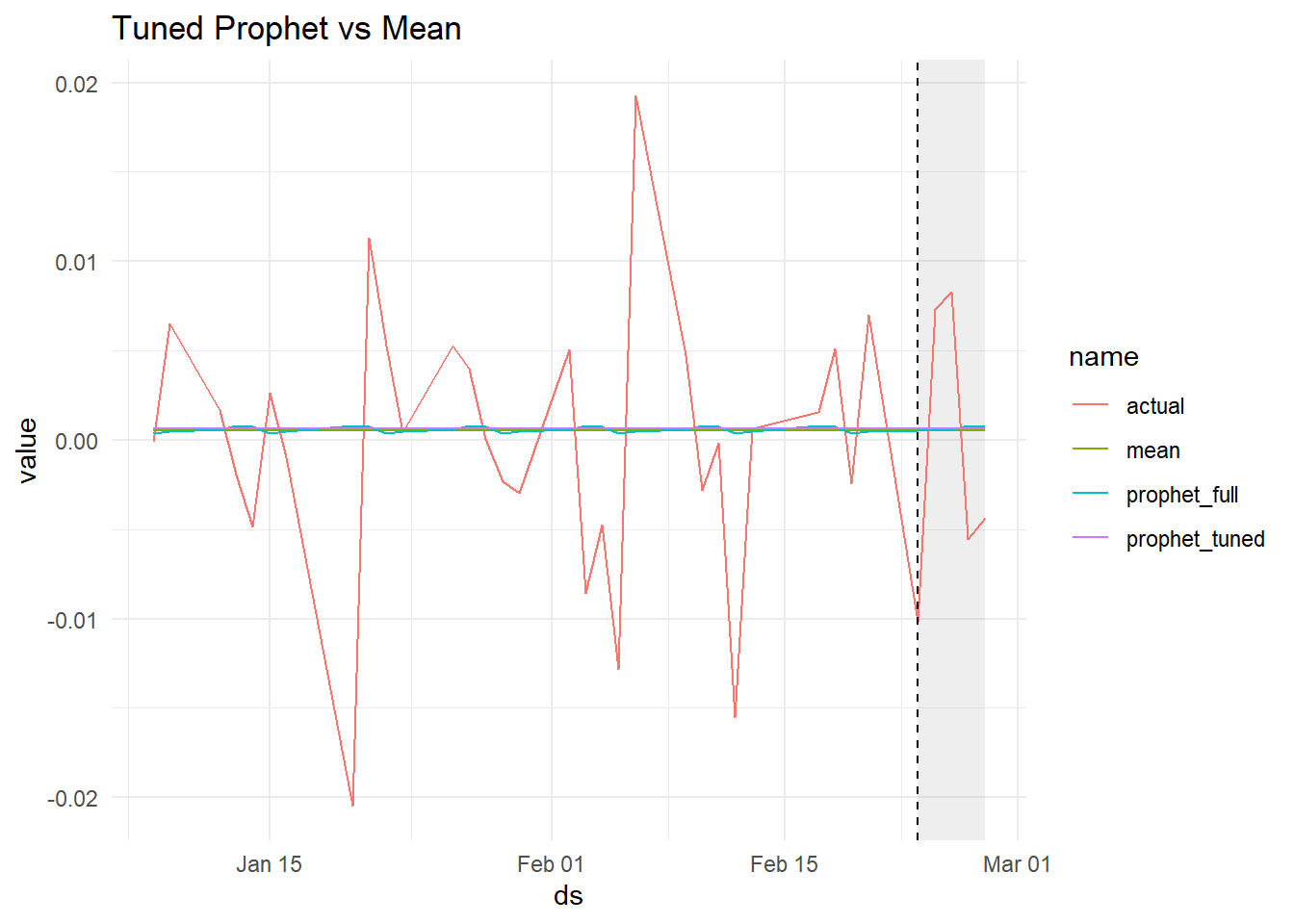
Task: plot some of the in sample and each of the out of sample results

plot_df$prophet_tuned <- c(
  tail(fc_best$yhat[1:nrow(train_full)], window_size),
  pred_best
)

plot_long <- pivot_longer(plot_df, -ds)

ggplot(plot_long, aes(x = ds, y = value, color = name)) +
  annotate("rect",
           xmin = cutoff_date,
           xmax = max(plot_df$ds),
           ymin = -Inf,
           ymax = Inf,
           alpha = 0.1) +
  geom_line() +
  geom_vline(xintercept = cutoff_date, linetype = "dashed") +
  ggtitle("Tuned Prophet vs Mean") +
  theme_minimal()

Q: Did tuning help?

A:

  • Not really.
  • Of course, we can do a full CV by rolling over multiple folds and searching a wider parameter space.
  • But if there is no (not much) trend/seasonality, Prophet is not going to provide reliable forecasts.